HanLe Liu ，QiYou Zhou ，GuoShan Li

Department of Earth Sciences Nanjing University, Han kou road #22, Nanjing 210093, China

Abstract:Most of organic pollutants belongs to LNAPL(Light Non-Aqueous Phase Liquid), leakage of which does serious contamination to soils and groundwater, and forms “water-LNAPL-air” three-phase system in the unsaturated zone. The purpose of our research is to investigate quantitative relation between electrical resistivity and each phase saturation in porous media. In the experiments fine sand and diesel oil were used. On the opposite two sides of the sand sample wall a total of eight stainless steel electrodes were settled at four different heights. By using a 12V, 10Hz alternative direct current as input, the voltage was measured by theWenner array method. For each sample box the calibration line between measured voltage and sample resistivity was obtained by using distilled water with different electrical conductance as sample and independently measuring the water resistivity with a Conductivity Meter. On the basis of a calibration line measured voltage was calibrated to the resistivity of the sand sample. The experimental results suggest that changes in water saturation or oil saturation will result in electrical resistivity variation in porous media, so it is possible to use electrical resistivity technique to monitor the saturation variation of water or LNAPL in “water-LNAPL-air” three-phase system.

Key words: LNAPL; organic pollutants; groundwater; porous media; saturation; electrical resistivity

1 Introduction

Leaks of hydrocarbons, such as Light Non-Aquous Phase Liquids (LNAPL) into the subsurface pose a serious risk of groundwater contamination. In order to obtain the success of remediation we must understand the subsurface distribution of LNAPL. As non-destructive and non-intrusive monitoring tool, Geophysical met-hods such as Electrical Resistivity Tomography (ERT), Ground Penetrating Radar (GPR) have been used to laboratory investigations and field observation at fuel spill sites, but there exist two conflicting viewpoints about geoelectric response of crude oil and refined product plumes.

Most of previous investigation support the model of high resistivity free phase (eg., Olhoeft,1992; De Ryck et al., 1993; Schneider et.al., 1993; Redman et al., 1994; Endes and Greenhouse,1996; Grumman and Daniels, 1996).

However, Gajdos and Kral (1995) reported resistivity decreases of 20% with the addition of about 1% crude oil to sand, and more than 40% resistivity decrease for a similar amount of motor oil. Similarly, Vanhala(1997) noted that the resistivity decreased in nearly every test sample of sands wetted with new motor oil or waste oil. Further, he observed that the decrease was maximum initially after adding the oil, but that the effect persisted until an oil content of 10% by volume was reached.

In order to undersatand the problem clearly, we have done a lot of experiments .There are three objectives of our study. Firstly, to understand how electric resistivity change with water saturation and LNAPL saturation in porous media. Secondly, to study electric properties of water-LNAPL-air system in different grain size porous media. Thirdly, to investigate the possibility using Electrical Resistivity Tomography (ERT) to monitor the saturation variation of water or LNAPL in multiphase system

2 Experimental Materials and Methods

2.1Experimental materials and procedure

Materials used in the experiment are distilled water, diesel oil and sand with four different grain size. The density of distilled water and diesel oil are 1.0 g/ml and 0.82g/ml respectively. Four different grain size are 0.45-0.9 mm, 0.3-0.45 mm, 0.2-0.3 mm, and 0.15-0.2 mm respectively. Sand sample box (height 6.5cm and internal diameter 4.5 cm) was made of acrylic pipe. On the opposite two sides of the box wall a total of eight stainless steel electrodes were settled at four different heights. By using the two electrodes at the same height as one electrode and a 12V, 10Hz alternative direct current as input, the voltage was measured by the Wennerarray method. Firstly, for each sample box the calibration line between measured voltage and sample resistivity was obtained by using distilled water with different electrical conductance as sample and independently measuring the water resistivity with a Conductivity Meter. Then, on the basis of a calibration line measured voltage was calibrated to the resistivity of the sand sample. Fig.4 shows calibration lines for sample box 2 and sample box 9. From the figure we can see that there is a linear relation between measured voltage and sample resistivity and we can obtain formula (1):

           ρ=k₁*V-k₂      (1)

whereρand V denote sample resistivity and measured water. k₁ and k₂ are calibration parameters for different sample box the calibration parameters are different. Table.1 summarize calibaration parameters for all box. From the table we can see that R² (correlation coefficient) are all near to 1,which suggest the linear relation are very well.

After establishing calibration lines we prepared different water saturation sand sample by mixing sand and water with different proportion. Then link apparatus like Fig.1. From Fig.2 we can see specific apparatus used in the experiment. Fig.3 shows the picture of sand sample.

2.2Experimental methods

For different experimental purposes three LNAPL dropping methods were adopted

Method # 1: Dropping 10ml LNAPL continuously.Method # 2: Dropping LNAPL continuously untill the sample become saturated

Method # 3: Dropping 2ml LNAPL every thirty minutes untill the sample become saturated

For method # 1, we prepared six sand samples whose water saturation are 0.09, 0.15, 0.21, 0.25, 0.32 and 0.37 respectiv-ely. The grain size of sand used is 0.3-0.45mm. For method # 2, we used two groups. As to group # 1, six sand samples were prepared, their water saturation are 0.07, 0.13, 0.20, 0.27, 0.37 and 0.47 respectively. The grain size of sand used is 0.3-0.45mm. As to group # 2 four sand samples were prepared, their grain size are 0.45-0.9 mm, 0.3-0.45 mm, 0.2-0.3 mm, and 0.15-0.2 mm respectively, and weight water content are all similar. For method # 3, twelve sand samples were prepared. Their water saturation are 0.11, 0.19, 0.27, 0.37, 0.45, 0.50, 0.37, 0.41, 0.45, 0.50, 0.56 respectively. The grain size of sand used is 0.3-0.45mm.

Fig.1 Experimental Setup

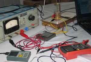
Fig.2 picture of apparatus

Fig.3 picture of sand sample

Fig.4 Calibration lines between voltage and electrical resisitivity

Table.1 Summary of calibration lines between measured voltage and sample resisitivity for all box

3 Experimental Results

3.1 Results of Method # 1

Fig.5 shows the results of method # 1. from the figure we can see that as LANPl dropping , for samples with low water saturation the resistivity change little, but for sample with middle and high obvious decrease for samples with higher water saturation. In this experiment ,LNAPL dropping velocity are different, so it may have some effect on the result. Fig.6 is the situation under similar dropping velocity. From the figure we can see water saturation the resistivity change much more and decrease at beginning, then increase. There appears the same phenomenon as Fig.5, for samples with middle and hight water saturation. The resistivety decrease at beginning then increase appear one critical point whose relative resistivity variation is minimum for fine grain, however, there appear one critical point whose relative resistivity variation is maximum for coarse grain.

Fig.5 Relative resistivity difference to variable LNAPL saturation of the sand sample with different water saturation

Fig.6 Relative resistivity difference to variable LNAPL saturation of the sand sample with different water saturation (under similar dropping velocity)

Fig.7 Relative resistivity difference to variable LNAPL saturation of the sand sample with different water saturation

Fig.8 Relative resistivity variation curves of sand sample with different grain size

3.3Results of Method # 3

For method # 3 , because the persistance time is longer ,the temperature may have effect on results. In order to get rid of this effect we have made temperature calibration. The calibration line can be seen from Fig.9. it illuminates that the resistivity decreeases according to temperature of sample and there exists linear relation between the resistivity and temperature. The relation can be described by formula (2):

ρ_r = -0.3562T_r + 0.0011    (2)

whereρ_r=(ρ_i-ρ₀)/ρ_{0 ,} denotes relative resistivity variation; Tr=(T_i-T₀)/T₀, denotes relative temperature variation

After making temperature calibration the change of resistivity according to LNAPL saturation and water saturation can be obtained. Fig.10 and Fig.11 illuminate relation curves between relative resistivity variation and LNAPL saturation for samples with low water saturation and high water saturation respectively. from these two figures we can see that the resistivity increases initially and than decreases for all samples, but theresistivity increases again for samples with low water saturation such as 0.11, 0.19, 0.27. for higher water saturation the resistivity decrease until samples saturated with LNAPL.

Fig.12 shows relation curves between resistivity and water saturation for samples whose LNAPL saturation are different. It is surprising to find that Archie’s [1942] formula described in formula (3) can be used to fit the data.

     (3)

Where ρ is the resistivity of the porous medium (Ωm), ρ₀ is the resistivity of the porous medium (Ωm) when S=1, β is a parameter related to the properties of the porous medium. The correlation coefficient fitting with Archie’s formula are near to one for samples whose LNAPL saturation are 0.28 and 0.66 respectively. while using Archie’s formula to fit the data of all samples with different LNAPL saturation the same surprising result can be obtained. Fig.14 illuminate the value of correlation Coefficient fitting with Archie’s formula according to LNAPL saturation ,we can see that correlation coefficient  are all between 0.95 and 1. therefore, at present of LANPL ,Archie’s formula can also fit the relation between resistivity and water saturation very well.

Since Archi’s formula can be used to fit the relation between resistivity and water saturation for samples with different LNAPL saturation, someone may ask how parameters of Archie’s formula change with LNAPL saturation. Fig.13 may give the answer. From this figure we can see that there are two critical points. The parameters ρ₀ and β keep constant generally when LNAPL saturation is less than 0.52, when LNAPL saturation is more than 0.52 and less than 0.66 the value of parameter ρ₀ will increase but the value of parameter β decrease. When LNAPL saturation is more than 0.66 the parameters ρ₀ and β keep constant again.

Fig.15 illuminate relative resistivty variation contours according to LNAPL saturation and water saturation. At the right area of the yellow line there is no data because the summation of water saturation and LNAPL saturation must be less than one. From this figure we can obviously see how relative resistivity variation change with LNAPL saturation for samples with different water saturation. There are one low value area and two high value area in the figure. While water saturation is low, as LNAPL saturation increase the resistivity increase initially than decrease, finally increase again. While water saturation is high, as LNAPL saturation increase the resistivity increase initially than decrease until samples become saturated with LNAPL.

4 Discussion

Shortcoming of the experiment is nonhomogenous distribution of fluids. LNAPL was input to porous media from the burette. At beginning, LNAPL was concentrated at the upper part of sand sample, as the amount increase LNAPL will infiltrate downwards due to gravity force. Before LNAPL was input water phase and air phase were uniformly distributed in the space of porous media. As we all know water phase exist in different form due to different water saturation. While satuation is low water phase is strongly absorbed on the surface of grain, therefore, LNAPL don’t affect water phase while infiltrating in porous space. However, while saturation is high water phase is0.52 and 0.66.

The mechanism described above can effectively interpret the result of method # 1 and method # 2. the result of experiment suggest that LNAPL and water belong to high resistivity phase and low resistivity phase respectively. for samples with low water saturation the resistivity shows low sensitivity to the change of LNAPL saturation. On the contrary, for samples with high water saturation the resistivity shows high sensitivity to the change of LNAPL saturation.not only absorbed on the surface of grain, but also exist in porous space. Therefore, LNAPL will depress water phase during the process of infiltration.

Fig.9 Temperature calibration curve

Fig.10 Relation curves between relative resistivity difference and LNAPL saturation of the sand sample with different water saturation (low water saturation)

Fig.11 Relation curves between relative resistivity difference and LNAPL saturation of the sand sample with different water saturation (high water saturation)

Fig.12 Relation curves between resistivity and  water saturation of the sand with different LNAPL saturation

Fig.13 Archie’s parameter curves according to LNAPL Saturation

Fig.14 Correlation Coefficient of Archie’s formula according to LNAPL saturation

Fig.15 Relative Resistivty Variation contours according to LNAPL saturation and water saturation

The result of method # 3 have illuminated how sample resistivity change according to LNAPL saturation and water saturation. For samples with different water saturation the relation between the resistivity and LNAPL saturation are different completely. While LNAPL saturation are similar the relation between sample resistivity and water saturation can be fit very well with Archie’s [1942] formula. It is surprising to find there is interesting relation between LNAPL saturation and parameters of Archie’s formula. For parameters of Archie’s formula there appears two critical point where LNAPL saturation are.

5 Conclusion

Water saturation has great effect on relative resistivity variation. As LNAPL saturation increases the variation of resisitivity is larger at high water saturation than at low water saturation in porous media. Therefore, it is better using ERT to monitor LNAPL saturation variation in high water saturation media than in low water saturation media

Grain size is also a great factor on relative resistivity variation. As LNAPL saturation increases, the resisitivity variation is larger in coarse grain than in fine grain

In water -LNAPL- air three-phase system Archie’s [1942] formula can also be used to fit the relation between resistivity and water saturation. For parameters of Archie’s formula it appears two critical point where LNAPL saturation are 0.52 and 0.66. While LNAPL saturation is less than 0.52 and more than 0.66, the parameter ρ₀ and β keep constant. when LNAPL saturation is in the range of 0.52 and 0.66, the parameter ρ₀decreases while parameter β increases. The specific reason for this phenomena will be investigated further in the future.

Acknowledgements

The authors wish to acknowledge Natural Science Foundation of China (40371021) for financial support and anonymous reviewer for helpful suggestions.

References

[1]      Archie, G. E., the electrical resistivity log as an aid in determining some reservoir characteristics, Trans. Am. Inst. Min. Metall. Pet. Eng., 146, 54-67, 1942.

[2]      De Ryck, S.M., Redman, J.D., annan, A.P., 1993. Geophysical monitoring of a controlled kerosene spill. In: Bell, R.S., Lepper, C.M. (Eds.), Proceedings of the Symposium on the Application of Geophysics to Engineering and Envionmental Problems (SAGEEP 1993), San Diego, CA, 5-20

[3]      Endres, A.L., Greenhouse, J.P., 1996. Detection and monitoring of chlorinated solvents by thermal neutron logging. Ground Water 34, 283–292.

[4]      Endres, A.L., Redman, J.D., 1996. Modelling the electrical properties of porous rocks and soils containning immiscible contaminants. Journal of Environmental and Engineering Geophysics 0 (2)., 105–112.

[5]      Olhoeft, G.R., 1992. Geophysical detection of hydrocarbon and organic chemical contamination. In: Bell, R.S. (Ed.), Proceedings of the Symmposium on the Application of Geophysics to Engineering and Environmental Problems (SAGEEP 1992), Oakbrook, IL, 587-595.

[6]      Schneider, G.W., De Ryck, S.M., Ferre, P.A., 1993. The application of automated high resolution DC resistivity in monitoring hydrogeological field experiments. In: Bell, R.S., Lepper, C.M. (Eds.), Proceedings of the Symposium on the Application of Geophysics to Engineering and Envionmental Problems (SAGEEP 1993), San Diego, CA, 145-162.

[7]      Redman, J.D., De Ryck, S.M., Annan, A.P., 1994. Detection of LNAPL pools with GPR: the Oretical modeling and surveys of a controlled spill. Proceedings of the Fifth International Conference on Ground Penetrating Radar (GPR 1994), Kitchener, Ontario, 1283-1294.

[8]      Gajdos, V., Kral, V., 1995. Influence of hydrocarb on pollution to soil conductivity. In: Bell, R.S. (Ed) Proceedings of the Symposium on the Application of Geophysics to Engineering and Environmental Problems (SAGEEP) 1995,  Orlando, FL,785–789.

[9]      Grumman, D.L., Daniels, J.J., 1996. Experiments on the detection of organic contaminants in the vadose zone. Journal of Environmental and Engineering Geophysics0 (1), 31–38.

[10]  Vanhala, H., 1997. Mapping oil-contaminated sand and till with the spectral induced polarization (SIP). method.Geophysical Prospecting 45, 303–326.