


Achievements
COMPOUND EFFECTS OF PARTIAL PENETRATION AND WEAKLY VERTICAL HETEROGENEITY ON THE ESTIMATION OF AQUIF
Chia-Shyun Chen1 ,C. G. Lan1, Jhong-Li2, Taoyuan2
1. Applied Geology Institute,
2.
Abstract:The partially penetrating effect induces vertical flow components in the neighborhood of the pumping well while vertical heterogeneity could alter an otherwise radial flow pattern throughout the aquifer. To investigate their compound effects on the estimation of aquifer transmissivity, a mathematical model is developed where the hydraulic conductivity is assumed to change exponentially with depth; an empirical relation determined using field data from multilevel slug tests. The solutions are determined using the Gram-Schmidt method due to the vertical heterogeneity involved. The partial penetrating effect is found to extend farther in a vertically asymmetric flow field than in a vertically symmetric flow field. The well discharge is under the influence of hydraulic conductivity as well as the flow pattern in the neighborhood of the well screen. The partial penetration effects could lead to an underestimate of transmissivity. Thus it is suggested that the pumping well fully penetrate the aquifer to minimize possible vertical heterogeneity effects.
Key words: partial penetration, vertical heterogeneity, constant-head pumping test, parameter estimation.
Introduction
It has been recognized that all natural formations are vertically heterogeneous to certain degree due to the depositional processes (Streltsova, 1988). The vertical sequence of deposits may be stratified as layers of high permeability alternating with layers of lower permeability. Many layered models have been developed, where the aquifers are assumed to consist of a number of layers of distinctive hydraulic properties [e.g., Li and Jiao, 2003; Hemker, 1999a, b, 1985; Streltsova, 1988; Javadel and Witherspoon, 1980; Wu, 1987; Gao, 1984; Prijambodo et al., 1985; Wikramaratna, 1984; Maas, 1987a, b, and others.]
Along with the advancement of the multi-level hydraulic tests [Melville et al., 1991; Butler et al., 2000; Zlotnik and Zurbuchen, 2003; Zemansky and McElwee, 2005], the hydraulic conductivity K can be determined at different depths with good resolution by using relatively small test increments. For example, Zemansky and McElwee [2005] conducted two multi-level slug tests to determine the vertical variation of K in an alluvial aquifer (Figure 1). One had a test interval of 0.15 m and the other of 0.61m. Both tests yielded consistent results, except for depth around 19 m where lower values of K were obtained by the test of the 0.15-m test interval. Ignoring this small discrepancy, it is found that the vertical variation of K can be relatively accurately approximated by
K() = K0exp(), 0 < < 1 (1)
where = z/b is the dimensionless depth with b being the total test depth, and = ln[K1/K0] is an empirical dimensionless parameter representing the strength of the vertical variability of K, and K0 and K1 are the hydraulic conductivities at = 0 and 1, respectively. If = 0, K does not change with depth and there is no vertical heterogeneity.
Many pumping wells only partially penetrate the aquifers. The partial penetration induces vertical flow components in the neighborhood of the pumping well [Hantush, 1964; Chen and Chang, 2003] while the vertical heterogeneity could alter an otherwise radial flow pattern throughout the aquifer. The purpose of this article is to investigate their compound effects on the estimation of aquifer transmissivity T based on the radial flow assumption. A mathematical model is developed for the conditions illustrated in Figure 2, where groundwater is withdrawn under constant drawdown from a partially penetrating well in a confined aquifer of vertical heterogeneity described by Eq. (1).The reason of using constant-drawdown pumping, instead of constant-rate pumping, is that the associate boundary condition can be unambiguously described by Eqs. (6) and (7) below. On the contrary, the boundary condition for constant-rate pumping in a partially penetrating well is subject to debate, as whether constant flux or constant head should be stipulated to the well screen [Hantush, 1964; Ruud and Kabala, 1997].
Model and Solutions
By reference to Figure 2, the confined aquifer is assumed to be isotropic, vertically heterogeneous as described by Eq. (1), of uniform thickness b, and of infinite areal extent. The dimensionless radial distance is denoted by r/rw); rw is the wellbore radius. The pumping well partially penetrates the aquifer with a screen length of s opened from t to b. Groundwater is withdrawn under a constant drawdown hwD = 1. The well discharge Qw() thus decreases with the dimensionless time = K0t/(Ssrw2), where Ss is storativity. The mathematical model in terms of dimensionless drawdown hD() is
![]() (2)
(2)
![]() (3)
(3)
![]() (4)
(4)
![]() (5)
(5)
![]() (6)
(6)
![]() (7)
(7)
where = rw/b. The involvement of e- on the right hand side of Eq. (2) makes the analytical solutions difficult to obtain. Given that e- varies in a narrow range between 0.9 and 1.0 for 0 < ≤ 0.1, this exponential term can be set to unity without introducing significant error, provided 0 < ≦0.1. As a result, Eq. (2) is modified as
![]() (8)
(8)
of which the analytical solutions are available. The successive applications of the Laplace transform with respect to and the separation of variables of and to Eq. (8) and Eqs. (3) to (5) result in
![]() (9)
(9)
where![]() ,
,![]() . For ≠ 0, the
infinite series in Eq. (9) is not a Fourier series and the coefficient Cn(p)
are not Fourier coefficients. They are determined here using the Gram-Schmidt
method [Kirkham and Powers, 1972; Chen and Chang, 2006]. This special technique
is particularly useful for approximating an analytical function using
non-orthogonal base functions, like the sine and cosine terms in the infinite
series of Eq. (9). In essence, Cn(p) are evaluated using the
Gram-Schmidt method to the result from applying Eq. (9) to Eqs. (6) and (7) in
the Laplace domain; the detailed discussion of
such practice is referred to Chen and Chang [2006]. It is noted that for = 0,
the infinite series in Eq. (9) becomes a Fourier series and Cn(p) should
be determined as Fourier coefficients with an appropriate method. In fact, the
solutions for = 0 were given by Chang and Chen [2003] and will be used below.
. For ≠ 0, the
infinite series in Eq. (9) is not a Fourier series and the coefficient Cn(p)
are not Fourier coefficients. They are determined here using the Gram-Schmidt
method [Kirkham and Powers, 1972; Chen and Chang, 2006]. This special technique
is particularly useful for approximating an analytical function using
non-orthogonal base functions, like the sine and cosine terms in the infinite
series of Eq. (9). In essence, Cn(p) are evaluated using the
Gram-Schmidt method to the result from applying Eq. (9) to Eqs. (6) and (7) in
the Laplace domain; the detailed discussion of
such practice is referred to Chen and Chang [2006]. It is noted that for = 0,
the infinite series in Eq. (9) becomes a Fourier series and Cn(p) should
be determined as Fourier coefficients with an appropriate method. In fact, the
solutions for = 0 were given by Chang and Chen [2003] and will be used below.
The constant-head pumping test is usually conducted as a single-well test, where the well discharge Qw(t) is measured and used in the specific drawdown to handle the parameter estimation [Chen and Chang, 2003; Chang and Chen, 2003; Jacob and Lohman, 1952]. In this sense, the specific drawdown is the ratio of the constant drawdown prescribed in the pumping well to the well discharge. The well discharge in the Laplace domain is
![]() (10)
(10)
where KD() = K()/K0 as the dimensionless hydraulic conductivity, and HD is defined by Eq. (9). The Laplace inversion of Eqs. (9) and (10) yields the depth-specific drawdown hD() and well discharge Qw(), respectively. The Stehfest [1970] method is used for evaluating the Laplace inversion.
Analysis and Discussion
The comparison of the depth-specific drawdown of = 0.1 and = 0 is demonstrated in Figure 3 for three cases, where a screen length of s = 0.2 is opened at bottom (b = 1 and t = 0.8), in the middle (b = 0.6 and t = 0.4), and at top (b = 0.2 and t = 0). It is understood that for = 0, the equipotential contours become exactly vertical where there is no partial penetration. For ≠ 0, however, the equipotentail contours under no influence of the partial penetration effect can only be “nearly vertical” due to distortion introduced by vertical heterogeneity. For = 0, the dashed equipotential contours in Figure 3b are symmetric with respect to the middle plane at = 0.5, and the dashed equipotential contours in Figure 3a and 3c are mutually symmetric with each other. The extent of the partial penetration effect is the shortest in Figure 3b. This is evidenced by the fact that the vertical dashed equipotential contour of 0.2 occurs approximately at ~ 155 in Figure 3b, while the vertical dashed equipotential contour of 0.15 occurs at ~ 250 in Figure 3a/3c.
For = 0.1, the solid equipotential contours in Figure 3b are almost vertically symmetric with respect to the middle plane of = 0.5. The solid equipotential contours in Figure 3a and 3c, however, are no longer symmetric with each other due to the vertical heterogeneity. The partial penetration extent is the shortest in the case of Figure 3b, where the nearly vertical solid equipotential contour of 0.15 takes place at ~ 190. In the other two cases, however, the nearly vertical equipotential contour of 0.1 occurs at ~ 315 in Figure 3a and at ~ 355 in Figure 3c.
The magnitude of the well discharge is under the influence of the hydraulic conductivity as well as the flow pattern in the neighborhood of the well screen. Figure 4 shows the well discharge, in terms of 1/Qw(), for the three cases studied in Figure 3. It is seen that the well discharge is influenced by K as well as the flow pattern in the neighborhood of the well screen. The largest Qw() is from the well screen opened in the middle, where the flow is most vertically symmetrical with respect to the center line of the aquifer while K is not the largest (from 9.17×10⁻⁴ to 5.12×10⁻⁴ m/s). The least Qw() is from the well screen opened at top, where the flow pattern is asymmetric either in the vertical or in the radial direction and K is the smallest (from 2.86×10⁻⁴ to 1.6×10⁻⁴ m/s).
The large-time asymptotic solution of the specific drawdown at the pumping well was given by Chen and Chang [2003] as
![]() (11)
(11)
where Ck is the pseudo-skin factor. This factor reflects head losses due to the partial penetration effect, the skin effect, and aquifer anisotropy. According to Eq. (11), plotting of specific drawdown versus logarithmic time would result in straight line at late times, and its slope m equals 0.183/T. Thus T can be estimated by
![]() (12)
(12)
Using Ss = 10-4 m-1, K0 = 10-5 m/s, b = 10m, hw = 2 m, and = 0.1, the hypothetical data of hw/Qw(t) are calculated based on Eq. (10) for the three cases and the case of a fully penetrating well. The semilog plot of these hypothetical data is shown in Figure 5, where the slope of each asymptote is indicated and the estimate of T given. The “true” transmissivity is thus
![]() (13)
(13)
It is seen that the partial penetration effect can lead to an underestimate of T. The estimate from the fully penetrating condition is closest to the “true” transmissivity.
Conclusion and Suggestion
The partial penetrating effect extends farther in a vertically asymmetric flow field than in a vertically symmetric flow field, and the compound effects of partial penetration and vertical heterogeneity aggravate the vertical asymmetry of the flow.
The well discharge is under the influence of K and the flow pattern in the neighborhood of the well screen.
To minimize the influence of possible vertical heterogeneity on the estimation of transimissivity, it is suggested that the pumping well be installed in a fully penetrating condition.
References
[1] Butler, J. J., Jr., A. A. Lanier, J. M. Healey, S. M. Sellwood, W. McCall, and E. Garnett, (2000), Direct-push Hydraulic Profiling in an Unconsolidated Alluvial Aquifer, Kansas Geol. Surv. Open-File Rep., 2000-62.
[2] Chang, C. C., and C. S. Chen, (2003), A flowing partially penetrating well in a finite-thickness aquifer: a mixed-type initial boundary value problem, J. Hydrol., 271, 101 - 118.
[3] Chen, C. S., and C. C. Chang, (2003), Well hydraulics theory and data analysis for the constant head test in an unconfined aquifer with skin effect, Water Resour. Res., 39(5), 1121, doi: 10.1029/2002WR001516.
[4] Chen, C. S., and C. C. Chang, (2006), Theoretical evaluation of non-uniform skin effect on aquifer response under constant rate pumping, J. Hydrol., 317, 190 – 201.
[5] Gao, C. T., (1984), Single-phase fluid flow in a stratified porous medium with crossflow, Soc. Pet. Eng. J., (February), 97 – 106.
[6] Hantush, M. S., (1964), Hydraulics of wells, in Advances in hydroscience, 1, edited by V. T. Chow, Academic Press, New York, 281- 432.
[7] Hemker, C. J., (1985), Transient well flow in leaky multiple-aquifer systems, J. Hydrol., 81: 111 - 126.
[8] Hemker, C. J., (1999a), Transient well flow in vertically heterogeneous aquifers, J. Hydrol., 225, 1 - 18.
[9] Hemker, C. J., (1999b), Transient well flow in layered aquifer systems: the uniform well-face drawdown solution, J. Hydrol., 225, 19 - 44.
[10] Jacob, C. E., and S. W. Lohman, (1952), Nonsteady flow to a well of constant drawdown in an extensive aquifer, Eos. Trans. AGU, 33(4), 559 - 569.
[11] Javandel, I., and P. A. Witherspoon, (1980), A semianalytical solution for partial penetration in two-layered aquifers, Water Resour. Res., 16(6), 1099 - 1106.
[12] Kirkham, D., and
W. L. Powers, (1972), Advanced Soil Physics, pp. 140- 159, Appendix 2, John
Wiley,
[13] Li, H. and J. Jiao, (2003), Tide induced seawater groundwater circulation in a multi-layered coastal leaky aquifer system, J. Hydrol., 274, 211 - 224.
[14] Maas, C., (1987a), Groundwater flow to a well in a layered porous medium 1. Steady flow, Water Resour. Res., 23, 1675 – 1681.
[15] Maas, C., (1987a), Groundwater flow to a well in a layered porous medium 2. Nonsteady multiple-aquifer flow, Water Resour. Res., 23, 1683 – 1688.
[16] Melville, J. G., F. J. Molz, O. Guven, and M. A. Widdowson, (1991), Multi- level slug tests with comparisons to tracer data, Ground Water, 29(6), 897 - 907.
[17] Prijambodo, R., R. Raghaven, and A. C. Reynolds, (1985), Well test analysis for wells producing layered reservoirs with crossflow, Soc. Pet. Eng. J., (June), 380 – 396.
[18] Ruud, N. C., Z. J. Kabala, (1997), Response of a partially penetrating well in a heterogeneous aquifer: integrated well-face flux versus uniform well-face flux boundary conditions. J. Hydrol., 194, 76 – 94.
[19] Stehfest, H. (1970), Numerical inversion of laplace transforms, Commun. ACM, 13, 47 - 39.
[20] Streltsova, T.D., (1988), Well
Testing in Heterogeneous Formations, An Exxon Monograph, John Wiley and
Sons,
[21] Wikramaratna, R. S., (1984), An analytical solution for the effects of abstraction from a multiple-layered aquifer with no cross flow, Water Resour. Res., 20(8), 1067 - 1074.
[22] Wu, S. Y., (1987), Steady ground-water flow through layered media, Transport in Porous Media, 2, 103 – 127.
[23] Zemansky, G. M. and C. D. McElwee, (2005), High-Resolution Slug Testing, Ground Water, 43(2), 222 - 230.
[24] Zlotnik, V. A., and B. R. Zurbuchen, (2003), Field study of hydraulic conductivity in a heterogeneous aquifer: Comparison of single-borehole measurements using different instruments, Water Resour. Res., 39(4), 1101, doi:10.1029/2002WR001415.

Figure 1. Vertical variation of K [from Zemansky and McElwee, 2005] approximated by K() = K0exp() with = 2.91 and K0 = 1.6×10⁻⁴ m/s.
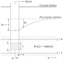
Figure 2. Schematic diagram of a partially penetrating well under constant-head pumping in a confined aquifer.
(a)
(b)
(c)
Figure 3. Drawdown contours determined by Eq. (9) of = 0 (dashed) and = 0.1 (solid) for three cases, (a) screen opened at top (t = 0 and b = 0.2), (b) screen opened in the middle (t = 0.4 and b = 0.6), and (c) screen opened at bottom (t = 0.8 and b = 1.0).
Figure 4. Well discharge in terms of 1/Qw() is plotted against logarithmic for the three cases studied in Figure 3. The largest Qw() is from the well screen opened in the middle, the least Qw() is from the well screen opened at top.
Figure 5. Hypothetical data of hw/Qw(t) versus logarithmic time for the three cases studied in Figure 3 and the case of a fully penetrating well.