Qingjun Zeng¹, Fang Xiao², Maoying Li²

1.South China University Of Technology., Guangzhou, 510640, China;

2.Department of Civil Engineering, Guangdong Communications Polytechnic, Guangzhou, 510650, China

Abstract: In this paper, the optimal management problems of water resource for a city of North China were discussed in the light of the thoughts of systematization, modeling, and optimization. Based on the mathematical simulation model of double-layer structure of the groundwater, a management model of the groundwater resource limited by certain groundwater level was established. At the same time, in accordance with long-term program of water usage, a multi-objective optimal management model used for the unified dispatching of the surface water and groundwater was also set up. Thus an multi-objective optimal distribution scheme of water resource was drawn out. The distribution scheme of water resource can directly satisfy the need of water resource management, and of establishment of some effective countermeasures on the continual usage of water resource.

Key words: Multi-objective optimization, Water resource management, System analysis, Continual development, Groundwater, Surface water.

1 Introduction

Deficiency of water resource or water supply is a pivotal factor of restricting the social and economical development. Continual development and usage of water resource is beneficial to the social and economical development, as well as protecting environment. In drought and semi-drought area of North China, reasonable development and scientific management of water resource and can effectively ease water resource crisis.

A city of North China, an industrial base of steel and machine, becomes the research area of this paper. In this area, exploitation of groundwater began in 1960’s. Excessive exploitation of groundwater and a great deal of polluted water which was discharged from industrial companies led to the continual decline of groundwater level and the worsening of water environment. Water dispatched from single well declined, and many driven wells were discarded as useless, which induced to the crisis of depletion of groundwater. In drought yeas, precipitation was very small by an average of 300mm a year. On the other hand, evaporative capacity was large. Continual aging of water conservancy facilities induced the decline of capacity of water supply. With the development of national economy, water demand is expanding rapidly, and the contradiction between water supply and water demand is becoming more and more incisive.

Water supply in the research area comes from surface water, groundwater and the Yellow River, as well as the polluted water. Surface water comes from seven valleys which traverse this area, with six dispatching works to make use of the Yellow River. The strategy of continual usage of water resource has been an important project with profound effect on the social and economic development. Generally speaking, there are some countermeasures, including developing new water source, optimizing the distribution of water resource, protecting water resource and mapping out related management rules as well as putting them into practice. This paper illustrated them from the point of optimizing the distribution of water resource, that is to say, how to carry out the optimal distribution scheme of water resource.

2 Numerical Simulation and Forecast of Groundwater System

Research area 1

Research area 2

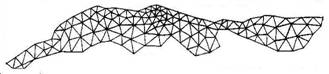
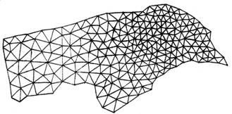
Fig. 1  Finite element meshes of phreatic and confined water aquifer

Based on the hydro-geologic and hydrological data of an area, numerical simulation describes quantitatively the relationships among factors consisting of groundwater system, and the intrinsic discipline of the system, consequently can lay a foundation for predicting of groundwater level and scientific management of surface water and groundwater resource.

2.1 Hydro-geologic model

The groundwater system in the research area is double-layer structure consisting of phreatic water aquifer, confined water aquifer and a clay layer existing between the two water-bearing layers. The area of phreatic water system is 1035.8 km2, while that of confined water system is 641.2 km2. According to geologic records, combining the sediment regular and rock properties of water-bearing system, water-bearing medium can be regarded as heterogeneous and isotropic medium. In addition, sub-precincts can be given according to the parameters of phreatic water aquifer and confined water aquifer. The hydrodynamic field were summarized as two dimensions non-stationary Darcy Flow Regime.

The study area was divided into two relative self-existent model areas—No.1 and No.2, according to the hydrogeology condition, as shown in Fig.1.

2.2 Mathematic formulation of simulation model of groundwater system

The double-layer groundwater model was established on the base of the hydro-geologic model, as given by

Where h1, h2 are the water level of phreatic water, and the artesian pressure respectively (unit: m); k1, k2 are percolation coefficients of the phreatic water aquifer and confined water aquifer respectively (unit: m/d); Q(h1,h2) is transfluence strength (unit: m3/d); ε is natural recharge strength of the phreatic water aquifer from the surface earth (unit: m3/d);  b is the elevation of the base plate of prelatic water aquifer (unit: m);  are the boundaries of the water level , water flow respectively; D1, D2 are the percolation areas of the prelatic, confined water aquifer respectively;  μ is water supply degree of the prelatic water aquifer; H01(x ,y),  H02(x, y) are the original water level of phreatic water aquifer,  and the original artesian pressure of confined water aquifer respectively (unit: m);  H(x, y, t) is boundary water level of the phreatic water aquifer (unit: m); q2(x, y, z) is unit wide flow rate on the lateral boundary of the phreatic and confined water system [unit: m3/(m. d)];  M is thickness of the confined water aquifer (unit: m).

2.3 Solving of simulation model of the groundwater system

Using finite element method, let partial differential equation (1) and (2) be discrete, we can get the matrix, as given by

Let ΔH=Ht+Δt-Ht, the equation can be expressed as given by

So we can get ΔH ,consequently Ht+Δt.

Dividing the whole calculating area into triangle in both No.1 research area and No.2 research area, we got 832 triangular elements, 472 nodes in No.1 area, 256 elements, 176 nodes in No.2 area. Marking the nodes in No.1 area and No.2 area as shown in Fig1.

Take time span from Oct. 1999 to Apr. 2000 as recognizing term, time span from Apr. 2000 to Oct. 2000 as testing term, which has experienced the hydrologic changes of a whole year. In the period between Nov. this year and April next year, there was no groundwater exploitation used for agriculture, avoiding statistic effects. Take one month as a calculating span.

This paper selected computer program compiled by professor Xueyu Lin in Jilin University, China [1].Adopting common methods, the hydrogeology parameter such as permeability coefficient, water supply degree, and etc were decided. The double-layer groundwater system model, which experienced many times by the way of reacting and debugging during inspection and recognition period, reflects the hydrogeology condition and becomes a base for forecasting the development of water regime and management of water resources.

2.4 Forecasting of the groundwater regime

(1) Original Flow Field and Forecasting Period

According to the development plan of this study area, this paper took 2004 year as the initial year, 2010 year as the forecasting year, one year as one period, then we got six periods altogether. Took the groundwater levels in Oct.2004 as the initial flow field.

(2) Forecasting Schemes

This paper selected two representative schemes to forecast the water regime. Scheme 1, with precipitation of assurance percentage 50%, the exploitation quantity used for industry and agriculture is equal to the practical value during one year, from Nov.2003 to Nov.2004. Scheme 2, with precipitation of assurance percentage 50%, the exploitation quantity used for industry and agriculture is equal to planning value during the forecasting future period.

(3) Determination of Boundary Conditions

The first grade of boundary conditions water level. The first grade of boundary conditions of prelatic water aquifer in research area is Yellow River level. The original data for forecasting the boundary water level all come from hydrologic station or inspection well laying on the bank of the Yellow River, altogether time span for six years. Since the length of the data series is short (n=6), then using gray model GM (1, 1) to forecast the first grade of water level on the boundary.

The method of determining boundary conditions of water flow in future is the same as that in the period for model recognition.

Forecasting of precipitation. Affected by weather factor, precipitation varies periodically. Its minimum is bigger than zero, but the maximum has no boundary.  According to the data of original precipitation from 1961 to 2000 in this area, we can predict the precipitation in different year in future period.

 (4) Forecasting Results and Some Relative Analysis

If we execute scheme 1, the value of accumulated usage of phreatic and confined water from now to 2010 year will be 5004×10⁴m³. If the scheme 2, the value will be 9005×10⁴m³, the phreatic water in some places will desiccate, and the line of confined water pressure will be lower than the elevation of upper plate of the confined water aquifer, consequently converting into no pressure state. So if keeping exploitation distribution at present, groundwater will be in serious over-mining state, whether exploitation as normal or according to the long-term.

3. Optimal Distribution of Water Resources

3.1 Dividing the study area into management sub-precincts of water resource

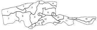
Fig. 2  Sketch map of sub-precincts for calculating management

The distribution of water resources is uneven, and groundwater is being exploited seriously, so the distribution scheme of water resource must be optimized. According to the properties of headwater and water usage, and considering the hydro geologic condition, this paper divided the research area into 16 sub-precincts as shown in Fig.2.

3.2 Optimal management model and distribution of water resource for groundwater system

(1) Management Scheme and Time Span

Assume the optimal management scheme of groundwater as following. Keep the existing exploitation distribution, consider water supply as the maximum at first, and the summation of all the drawdown of water level as the minimum.

Time span of management is from 2004 year to 2010 year, one year as a period.

(2) Setting up Decision Variables

In the sub-precincts, exploitation quantity of phreatic water used for industry was designated as Xi (i=1, 2, …., L); that of phreatic water used for agriculture is designated as Xi(i=L+1….2L);that of confined water used for industry is designated as Xi(i=2L+1,…,2L+L1);that of confined water used for agriculture is designated as Xi(i=2L+L1+1,….,2L+2L1); that of each triangle element is designated as Xi(i=LM+1,…,LK); assurance percentage of water supply for industry is designated as Xi (i=LK+1,….,LK+L); assurance percentage of water supply for agriculture is designated as Xi (i=LK+L+1,….,K1).

Where LM=2L+2L1, LK=LM+MD, K1=LK+2L, L (=16) is the number of total sub-precincts for calculating management, L1 (=11) is the number of sub-precincts with double-layer structure including both phreatic water aquifer and confined water aquifer, MD is the number of strong pumping elements, K1 is the number of total decision variables.

(3) Multi-objective Function for Optimization

According to the management scheme, there are three grades of target layers which are water supply for industry as the maximum first, water supply for agriculture as the maximum second, and the summation of all the drawdown of water level as the minimum third. So the multi-objective weighting function of management is given by

Where ,,are the weights,=0.645，  =0.2966，  =0.0584 (By Seaty’s mathematical method); NP is the number of calculation nodes; Sj are the drawdown of water level of calculating nodes, which can be expressed as the function of variable Xi (i=1, …., K1), j=1,…,NP.

(4) Limited Conditions

It mainly consists of limitation of groundwater level, supply-demand limitation of groundwater resource and limitation of phreatic water considering environment protecting. Drawdown of water level can be expressed as the function of variable Xi (i=1, …., K1).

(5) Improvement of Optimal Model and Calculation of Response Coefficient

One part of multi-objective weight function depends upon assurance percentage of water supply, the other depends upon drawdown of water level. One part of decision variables depend upon assurance percentage of  water supply, while the other depend upon water quantity. One part of limited conditions also depend on drawdown of water level, the other depend on water quantity and assurance percentage of water supply. Therefore, if the drawdown of water level can be expressed as water quantity, then we can only use water quantity and assurance percentage of water supply to describe optimal model. Drawdown of water level must be converted into the function of water quantity by means of numerical methods, generally, adopting response matrix to solve the problem.

Equation (2) is linear, but equation (1) describes a non-linear system. In order to make equation (1) linear , assume that water level of phreatic water aquifer varies relatively little, regard that water transmissibility coefficient (T1) is constant as given by

T1=K1(H01-b)=K1M1

Where Ho1 is phreatic water level of Nov.2004.

Thus, both equation (1)and (2) become linear. System input are divided into two parts, one is (P1,P2) affected by men, the other is [Q(h1, h2)，ε ] affected by nature. Input the two parts respectively and sum up the results respectively obtained from output system, then get the output results of the original system.

For example, assume that groundwater is pumped from element i, then the drawdown of node j in 2010 will be given by

   (4)

Where i=1,…, I(I is the number of pumping elements); j=1,…, J(J is the number of total nodes); k=1,2…,K (K is the total periods of pumping, here K=6); β(i, j, K-k) is response coefficient to unit pulse; S(i, j ) is the drawdown of node j in 2010 induced by pumping from element I; Q(i, k ) is pumping water quantity from element i in period k.

(6) Running of Optimal Management Model and Analysis of Its Results

LP management model established in this paper is a linear planning problem, in which there are 322 decision variables, the number of limited conditions are 273, we can use simplex method to solve the equation. Interaction of numerical model established by finite element method and optimal model can help us accomplish successfully the optimizing distribution of water quantity in the groundwater system.

Solve the LP management model, then we can get the maximum value of assurance percentage of water supply, optimal exploitation quantity used for industry and agriculture in every sub-precinct, shown in Table 1, and the contour map of water level of phreatic and confined water aquifer at the end of management term, which are omitted here.

Table 1 Optimized exploitation quantity of groundwater used for industry and agriculture of every sub-precinct in 2010

1        0      754.33     0         0       754.33     100

2      46.06    417.12    148.51     0       611.691     100

3     1071.01   335.41    504.55    25.12    1936.09     100

4     908.34    419.52    1530.21   226.71   3084.78     100

5     59.02     153.62    425.62    68.11    706.37      100

6     569.71    1875.01   124.82    328.25   2897.79     100

7       0       102.45      0       0.09     102.54     100

8       0       207.31      0       15.61    222.92     100

9      4.1      3.10      8.71        0       15.91     100

10    493.12    436.11    168.22    14.32   1111.77      100

11    30.00     935.26      0       13.82    979.08     100

12      0      147.25       0         0      147.25    100

13      0      97.82        0         0      97.82     100

14    1.23     2589.81      0         0      2591.04   100

15    1120.23   451.88      0         0      1572.11    100

16    43.24    1850.33      0         0      1893.57    100

G.T.  4346.07   10776.33   2910.64   692.03  18725.07

From Table 1, we can know that the ratio between exploitation quantity of phreatic water and that of confined water has been adjusted from 2.44:1.00 in 2004 to 4.2:1.0 in 2010. As far as hydrodynamic field is concerned, the drawdown of more than half of nodes of phreatic water aquifer are lowered than 0.5m a year, and the water level of most nodes of confined water aquifer can be recovered, which is beneficial to the environment protection of.

3.3 Unified Optimal Management Model and Optimal Distribution of Surface Water and Groundwater

(1) Meaning of Unified Optimal Distribution of Surface Water and Groundwater

Water demand used for industry and agriculture rises rapidly, and that in 2010 year is two time as much as that in 2005 year. Optimal management model of groundwater quantity can only resolve problems such as groungwater desiccation in some nodes on account of unreasonable distribution of exploitation. But if we only optimize and adjust the ground system, we still can’t easily resolve the existing problems and contradictions between supply and demand of water resources in research area. So it is the unique key way to establish a unified optimal model among groundwater, surface water system and water demand system, combining the total water quantity required in research area in 2010.

(2) Determination of Management Scheme

Assume the unified optimal scheme of groundwater and surface water as following: Based on exploiting groundwater uniformly, consider deficiency of water for industry as the minimum first, that for agriculture as the minimum second, and total exploitation quantity of groundwater as the minimum third, make best use of surface water, and meet the need of preventing environment.

(3) Time Span and Scope of Management                                   

Management period, scope and its sub-precincts are the same as management model of groundwater system.

(4) Setting up decision variables

For every precinct, exploitation quantity of phreatic water used for industry are Xi (i=1,……L), that of phreatic water used for agriculture are Xi (i=L+1,…2L),that of confined water used for industry are Xi (i=2L+1,……2L+L1 ),that of confined water used for agriculture are Xi (i=2L+L1+1,…,2L+2L1 ); exploitation quantity of groundwater of triangle elements are Xi (i=LM+1,…,LK ); existing surface water used for industry are Xi (i=LK+1,…,LK+5) which supply five sub-precincts 3,4,9,10 and 15; that of water dispatched from new works constructed along Yellow River are Xi (i=LK+6,…,LK+10) which supply five sub-precincts 4.5,9,10 and 15 used for industry, that of surface water used for agriculture irrigation are Xi (i=LK+11,…,LK+16 ) which supply five sub-precincts 1,7,8,11and 16; water deficit for industry of each precinct are Xi (i=LK+17,…,LK+16+L), water deficit for agriculture of each precinct are Xi ( =LK+17+L,…,K1). Where LM=2L+2L1,LK=LM+MD,K1=LK+16+2L, their meanings are the same as management model of groundwater system.

(5) Multi-objective Optimal Weight Function of Management

According to management scheme, consider deficiency of water for industry as the minimum first, that for agriculture as the minimum second, and total exploitation quantity of groundwater as the minimum third, the multi-objective weighting function of management is given by

Where  ,  ,  are the weights,   =100,  =10,  =1 because of letting the weight value of the highest priority equal to 100, that of higher equal to 10.

(6) Limited Conditions

It consists of limitation of water level, groundwater supply and surface water supply.

3.4 Running of Unified Optimal Management Model and Optimal Distribution Scheme

There are 344 decision variables, 291 limitation conditions in all in the linear planning model, and the problem can be resolved by simplex method.

Running the unified optimal management model, we can obtain optimal exploitation distribution of groundwater of each sub-precinct as shown in Table 2, and related optimal water level in 2010 as ignored here. We also know that optimal surface water distribution of each sub-precinct shown in Table 3, the water deficit for industry is 0, while water deficit for agriculture is 2657.64×104m3, water deficit of sub-precincts from 1 to 16 are ( 667.98 , 256.77, 128.38, 346.17, 9.15, 449.55, 0, 0, 5.02, 14.40, 0, 0, 0, 555.64, 224.58, 0 ) ×104m3 respectively.

(1) Analysis on Optimal Supply-Demand of Water Resource

Water deficit for industry and agriculture: Water supply meets the demand for industry with priority, so the water deficit of all the calculating sub-precincts are zero. On the other hand, for agriculture, there are 10 calculating sub-precincts lacking of water in different degree.

Table 2  Unified optimal exploitation quantity of groundwater used for industry and agriculture of every precinct in 2010

    1         0      665.32     0         0       665.32    

    2       47.01    190.21    295.71     0       532.93   

    3      283.92    185.25    234.68   138.25    842.1

    4      119.25    217.77    969.23   179.11    1485.36

    5      7.11      148.21    182.65   85.81     423.78

    6      740.54    1282.01   654.23   736.33    3413.11

    7        0       101.56      0      0.09      101.65

    8        0       271.55      0      12.45     284.00

    9       0.67     1.22      2.85        0      4.74

    10     107.70    442.31    82.72    47.85     680.58

    11     34.51     451.31      0      60.26     546.08

    12       0       185.70      0         0      185.70

    13       0       119.20      0         0      119.20

    14     4.81      1945.24     0         0      1950.05

    15     255.22    420.77      0         0      675.99

    16     18.12     2029.18     0         0      2048.45

    G.T.   1618.86   8656.25  2422.07   1260.21    13957.95

Table 3  Unified optimal exploitation quantity of surface water used for industry and agriculture of every precinct in 2010

    1    0           0          418.20    418.20    0

    2    0           0          0         0         0

    3    29128.22    0          0         29128.22  192.2

    4    2546.28     10944.14   0         13490.41  717.66

    5    0           4348.68    0         4348.68   42.69

    6    0           0          0         0         1211.94

    7    0           0          2839.85   2839.8    0

    8    0           0          1741.95   1741.45   0

    9    5.74        160.08     0         165.82    40.82

    10   182.93      4939.89    0         5122.82   20.00

    11   0           0          1847.00   1847.00   40.72

    12   0           0          0         0         0

    13   0           0          0         0         0

    14   0           0          0         0         515.31

    15   1636.43     0          0         1636.43   100.00

    16   0           0          1209.00   1209.00   0

    G.T.  33499.60    20392.78   8056.00   61948.38  2871.44

Reasons of water deficit for agriculture are that water supply of surface water rises a little in 2010 year, and groundwater, especially confined water, meets the demand for industry with priority. Though the united optimal management model of surface water-groundwater system would been executed, it still can’t meet the demand because of the uneven distribution of water resources.

(2) Analysis on Optimal Groundwater System

Total exploitation redistribution of groundwater: use surface water at first when surface water is ample and exploit groundwater in a little degree, saved groundwater will supply the elements with water deficit and no surface water supply, which shows the principle of unified optimization.

The drawdown of more than half of nodes of phreatic water aquifer are lower than 0.5m a year, and the water level of most nodes of confined water aquifer can be recovered, which is beneficial to the protection of environment.

(3) Analysis on Optimal Surface Water System

Total optimal water quantity used for industry from other surface water supply works is 33499.6×104m3, which is up to top limit of supply work. So in 2005 year some sub-precincts such as No.4, 10 should use water dispatched from new Yellow River works in order to reduce the exploitation of groundwater especially confined water.

(4) Strategy of Resolving the Problem of Water Deficit for Agriculture

How to solve the problem of lacking of water for agriculture in 2010? Reasonable distribution of industrial structure, and developing thrift agriculture can ease water deficiency. In the agricultural planting area of sub-precinct 3, 4, 5, 6, 9, 10, 15,, water demand are almost all dispatched from groundwater. So advise to convert vegetable planting area, which need a great deal of water, from sub-precincts with over-exploitation of groundwater to other sub-precincts with relatively ample water source, such as sub-precincts 1, 14, 8 , 13, 16 in order to reduce the exploitation of groundwater.

4  Conclusions

(1) This paper employed the view of system engineering, dynamic analysis, and computer simulation to analyze the problem of optimal distribution scheme of water resource in research area.

(2) Running the mathematical simulation model of double-layer structure of the groundwater, the groundwater may seriously be over-exploited whether in the present exploitation state or in the planning exploitation state, which must be controlled.

(3) In order to meet the water demand for industry first, for agriculture second, and to develop groundwater and surface water in unit, an optimal management model used for the unified dispatching of the surface water and groundwater was set up in accordance with long-term program of water usage. Thus an optimal distribution scheme of water resource was drawn out.

(4) Including putting a unified optimal distribution scheme of water resource into practice, there are also some key measures such as developing thrift agriculture and industry rapidly, protecting water resource from pollution and constructing new hydro conservancy engineering in order to assure the continual usage of water resource in the study area.

References

[1]      Xueyu Lin (1988). A collection of management and computer simulation program for quantity and quality of    groundwater. Jinlin Publishing House of Science and Technique, Changchun, China.

[2]      Yidong Lin, Baozhu Sun, Lirong Lin (1993). Engineering hydrology. Publishing House of Hohai University, Nanjing, China.

[3]      Yunwei Sun, Haijun Yan (1990). System structure of water resource. Proceeding of IAHS