Evolutional Rules of Regional Groundwater System
RESEARCH ON DYNAMIC OBSERVATION FREQUENCY OF GROUNDWATER LEVEL BASED ON THE ANALYSIS OF TIME SERIES
Li Changqing1, Xu Yanze1, Jin Ping2
1. China Institute of Geological Environmental Monitoring, Beijing, 100081;
2. PAIDE TM Information Technology Co. Ltd., Beijing, 100085
Abstract: Based on the three characteristics of groundwater level fluctuations, including certainty, periodicity, and randomicity, the method of time series analysis is used to study them in the paper. The equation of groundwater level series is divided into trend items, periodic items and random items on the basis of polynomial and Fourier series. Therefore, the observation interval in the different width of confidence interval can be calculated by analyzing the three items under some restrained conditions. In the end, the realization and evaluation of the method is shown one by one in the paper.
Key Words: the optimization of observation frequency, time series analysis, polynomial, Fourier series, confidence interval width.
1 Introduction
Time series refer to a sequence of random variation on time order. Any series become the composition of three parts by reasonably changing some function, including trend items, periodic items and random items [1]. Therefore, it is primary to decompose time series into these three items. The analysis of time series is an applied branch of probabilistic and statistical science, being used widely in plenty of fields such as financial economy, meteorological hydrology, signal disposal, and mechanical librations.
Nowadays, groundwater level is usually observed every five days in most places in China except that automatic monitors are used in a few areas, their observation frequency up to each one hour and even more. Obviously, the values of groundwater level monitored corresponding to the definition of time
series can be regarded as a random variable sequence
on some time series, because groundwater level fluctuation is continuous in nature but represents discrete on the interruption of human activity. A continuous sequence can be simulated by discrete data, which accuracy is determined by time interval of these data. The shorter time interval is, the more accurate actual series are simulated.
The variation of groundwater level is complex on the restriction of kinds of factors, so the relation among them is difficultly grasped. The research on dynamic series of groundwater level found there were some uncertain factors leading to groundwater level fluctuation that might be caused by observation errors or the influences of specific geographic, geological and meteorological condition even or some elements undiscovered by people. To some extent, however, these factors have certain, periodic and random characteristics. Precipitation and evaporation have a periodic impact on groundwater level fluctuation. The effects of manual extraction and agricultural irrigation on the level are rather certain. Some natural factors such as crustal movement and tide and human factors like observation errors prefer to randomicity. Therefore, the fluctuation of groundwater level has the features of certainty, periodicity and randomicity due to the effects of factors motioned above together on the fluctuation.
Considering certainty, periodicity and randomicity of groundwater level, using the analytic method of time series can optimize observation frequency. The method belonging to probability and statistics is used widely in many fields. The main steps are to separate time series into trend items, periodic items and random items and constitute a relative suitable statistic model. To any time series, the three items can be obtained by reliable function change, respectively reflecting the characteristic of certainty, periodicity and randomicity.
2 The Basic Principle to Optimize Observation Frequency
The optimization of dynamic observation frequency of groundwater level has been studied a lot in the world, introducing many methods such as Kringing, Kalman’s filteration and optimum model. It is noted that Wu Yanqing, Li Junting, Wang Wenke and et al. did significant contributions on the field in China [2, 3]. The analytic method of time series was used to optimize observation frequency of groundwater level by some studied persons, the result almost tending to only one value. In the paper, trend, periodic and random items separated from the sequence of groundwater monitored would be analyzed by using time series, resulting in observation frequencies in different confidence interval widths.
In the progress, the influence of certainty factors (been regarded as trend items) is removed firstly from a dynamic sequence of groundwater real level. The residual sequence (including periodic and random items) is analyzed periodically according to Fourier series method, disposing of periodic items. By studying the residua being thought of as random items, observation frequency can be determined under the requirement of some condition and accuracy. Supposing Ht is an actual sequence of groundwater level monitored, the total number of samples is n, and observation interval is △ with the unit of day, so an equation can be written as
![]() (1)
(1)
where Ht is a dynamic sequence of groundwater level monitored, and Tt is trend sequence of groundwater level, and St is periodic sequence of groundwater level, Rt is random sequence of groundwater level.
2.1 The analysis of trend items (Tt)
Due to trend items with certainty, they can be expressed in equations from the aspect of statistics and their variation is certain. The aim is to remove the items from the sequence of groundwater level monitored by analyzing them. There are many dissolved methods, including polynomial and curve analysis. The former is composes of simple (linearity), quadratic and cubic polynomial and so on. The latter mainly contains exponential and logarithmic curve. Comparing and contrasting these two methods, polynomial is universal because any curves can be simulated by it. According to the results of several tests, the polynomial is usually applied no more than quintic one, in which trend items can be removed from the real dynamic observation sequence.
![]() (2)
(2)
![]() ,
,![]() ,
,![]() …
…![]() represent polynomial coefficients.
The coefficients could be calculated by using the method of minimum square
approaching in orthogonal polynomial (also called as minimum square simulation
in orthogonal function)[4], which is the best fitting method in
simulating curves [5]. The progress to obtain function (2) is not
explained in detail. From function (2), trend items are just a time function.
If time is determined, observation time of groundwater level is decided, trend
items being confirmed as well. Whether the frequency is big or small, the items
are hardly affected. Therefore, the items are only related with time variable,
having few impacts on optimizing observation frequency of groundwater level.
represent polynomial coefficients.
The coefficients could be calculated by using the method of minimum square
approaching in orthogonal polynomial (also called as minimum square simulation
in orthogonal function)[4], which is the best fitting method in
simulating curves [5]. The progress to obtain function (2) is not
explained in detail. From function (2), trend items are just a time function.
If time is determined, observation time of groundwater level is decided, trend
items being confirmed as well. Whether the frequency is big or small, the items
are hardly affected. Therefore, the items are only related with time variable,
having few impacts on optimizing observation frequency of groundwater level.
2.2 The analysis of periodic items (St)
Following the elimination of trend items from an observation sequence of groundwater level, Fourier series are used to analyze the periodicity of the residual series(Ht-Tt) Xt is residual sequence and n is the total amount of samples.
![]()
(i=1,2,3,…,n) (3)
where i is the number of sample, and s(i)is the value in the periodical item of sample i, and j is harmonics, and b0,bj,cj is the coefficients of Fourier.
In minimum square function, the values of b0, bj, cj estimated impartially are:
![]()
![]()
![]() (j=1,2,3,…,m) (4)
(j=1,2,3,…,m) (4)
m is the number of harmonics. It is shown in function 3 that the periodical items St become closer with the residual sequence Xt with the numerical increase of harmonics (m). However, the bigger of harmonics (m) does not mean better. Because random items(Rt)is objective, the number of harmonics (m) can reach the requirement of periodic analysis just when the items satisfy some condition (independent and standard deviation less than 0.5).
The physical meanings of Fourier series show that periodical items are the superimposition of the number (m) of harmonic. Every harmonic can be expressed in function 5.
![]() (5)
(5)
where A0 is
constant,representing the weight of
direct current in electro technician;and
A is amplitude, and ω is angular frequency, and ![]() is the initial value.
is the initial value.
Fourier series are superimposed by a certain number of sinusoid or cosines curves (just being harmonic). Each harmonic with an unknown coefficient, the coefficient can be determined by at least four known data. In function 3, the number of data equal to multiply four by m, realizing the numerical demand of data in the trend analysis.
To clearly reflect the periodical requirement of time series, observation interval is decided in function 6.
![]() (6)
(6)
where KS is observation interval corresponding to periodical items. It is shown in function 6 just by analyzing periodical items of time series that the more is the number of harmonic at the same period, the less is observation interval and otherwise the less is the number, the more is the interval.
2.3 The analysis of random items (Rt)
Groundwater system is parts of the whole water circulatory system, definitely being affected by surrounding environmental. Because these effects are random, the randomcity of groundwater level is objective. In additional, it is inevitable that observation value of groundwater level is different from real value under the restriction of measuring technique, methods, equipments and so on when human being pumps groundwater. The difference is random, so random items have to be paid attention on optimizing observation frequency of groundwater level.
The items (Rt) are time sequences after the extraction of trend and periodic items from real observation series. Supposing random items belong to normal distribution. They have to satisfy the requirements mentioned below:
(1)Random items are independent. In monitoring groundwater level, the relative data sequences have less information than the independent.
(2)Their standard deviation is less than 0.5.
(3)The confidence equaling to 95%, the average of random items need satisfy the confidence interval width given.
It is judged firstly whether random items are independent or not.
According to District function [6],when an autocorrelation coefficient satisfies function 7,
![]() (7)
(7)
where n is the number of data, the probability of the coefficient equaling to zero is 95%, the data sequences being independent. Then the average of random items can be calculated in function 8.
![]() (8)
(8)
When random items are
independent sequences, var(![]() )=σ2/n(σ2 is total deviation, which can be replaced similarly by
Sample variance with the large number of sample).The
average of samples being at the 95% of confidence, the confidence interval is:
)=σ2/n(σ2 is total deviation, which can be replaced similarly by
Sample variance with the large number of sample).The
average of samples being at the 95% of confidence, the confidence interval is:
![]()
The confidence interval width is:
![]() (9)
(9)
where N is observation times satisfying the demand of random items in the certain confidence interval width given. Under the requirement of random items and confidence interval width determined, observation interval KR is:
![]() (10)
(10)
3 The Determination of Observation Interval
By analyzing periodic and random items, observation interval of groundwater level(K)is the minimum of Ks by periodic analysis and KR by random analysis under the certain confidence interval width and at 95% of the confidence. Function 11 is:
K=min(KS,KR) (11)
4 The Steps to Optimize Observation Frequency
By concluding the analysis above, the optimizing progress is:
(1)Clearing up real observation data of groundwater level. The method requires the observation data are sequences in certain time interval. Interpolation method is used to fill up the individual absent data of groundwater level, obtaining the observation sequences of groundwater level.
(2)Simulating by polynomial. Minimum square method is employed to simulate Ht and calculate the uncertain coefficient, resulting in trend items Tt and the residual sequences Xt.
(3)Analyzing periodicity. Fourier series are used to analyze the periodicity of the residual sequences. On the usage of function 4, Fourier coefficient can be obtained in the meaning of Minimum square method.
(4)Analyzing independent condition. Resumed the number of harmonic (I) being 1, the periodic items St and the random items Rt can be calculated in function 3. Then the random is estimated whether they satisfy function 7 and their standard deviation is less 0.5. If they are not, the number of harmonic (I) need to add one and recalculate the random until the items reach the requirements. At that moment, I is the suitable number of harmonic. Observation interval Ks can be obtained by function6.
(5)Analyzing random items under the certain confidence interval width. Observation interval KR can be obtained in function 9 and 10 under the demand of random items Rt in term four above and of the certain confidence interval width.
(6)Determining the optimum observation interval. The optimum observation interval satisfying all conditions is decided by function 11 under the certain confidence interval width.
5 Studied Cases and Conclusions
5.1 Analyzing time sequences of monitored data
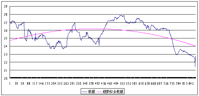
Computer programming language realizes the optimization of observation frequency of groundwater level above and is employed in the study of Huabei Plain. For example, the monitoring well with the number of 1101010001 has observation sequences of water level from 1993 to 2004, totaling 864 data during 12 years. Its monitoring frequency is every 5 days.
As Figure 1 is shown, observation data(Ht)was simulated by using quadratic polynomial. The polynomial simulated is T(t)=24.712+0.00758×t-0.00000973×t2. Trend items (Tt)was eliminated from monitored data(Ht), obtaining the residual sequences(Xt).

Figure 1. The simulated curve of trend items(Tt)based on observation data of water level
Periodical analysis was cited in the residual sequences(Xt)by using Fourier series, obtaining Fourier coefficients (which are not listed in detail because of plenty of data ). When confidence interval width is 0.05m and the standard
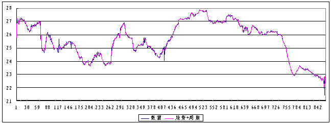
deviation of random items is less than 0.5m, the periodical (St)and random items(Rt)can be simulated as in figure 2 and 3. It is shown that Figure 4 is the superimposition curve of the trend and periodical items(Tt+St)by comparing the curve of observation data of water level.

Figure 2. The curve of periodical items(St)based on observation data of water level

Figure 3. The curve of random items(Rt)based on observation data of water level

Figure 4. The compared curves of the superimposition(Tt+St)of trend and periodical items and observation data(Ht)
5.2 Optimizing observation frequency
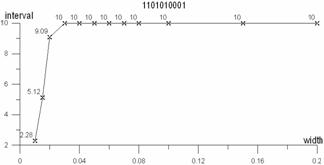
Using the analytic results of time series, the optimum observation intervals(K)are calculated when the confidence interval widths respectively are 0.005m, 0.01m, 0.015m, 0.02m, 0.03m, 0.04m, 0.05m, 0.06m, 0.07m, 0.08m, 0.10m, 0.15m, and 0.20m. They are shown in table 1 and figure 5.
Table 1. The optimum observation intervals in different confidence interval widths
|
confidence interval widths(m) |
optimum observation intervals(d) |
confidence interval widths(m) |
optimum observation intervals(d) |
|
0.005 |
0.06 |
10 | |
|
0.01 |
2.28 |
0.07 |
10 |
|
0.015 |
5.12 |
0.08 |
10 |
|
0.02 |
9.09 |
0.10 |
10 |
|
0.03 |
10 |
0.15 |
10 |
|
0.04 |
10 |
0.20 |
10 |
|
0.05 |
10 |


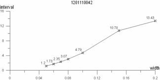
Figure 5. The relation between optimum observation Figure 6. The relation between optimum observation
intervals and different confidence interval widths 1 intervals and different confidence interval widths (2)
In figure 5 and 6, the abscissa reflects confidence interval width (the unit is m), and the ordinate is observation interval (the unit is d). The two figures shows
(1) Different confidence interval widths correspond to dissimilar observation intervals. If a confidence interval width is small, the observation interval is low. Otherwise if a width increases, the interval shows linear augmentation. It is obvious that the items have positive relation, being similar with common sense.
(2) The increase of observation intervals is not unlimited, being stable at some observation intervals due to the periodical characteristics of groundwater level sequences. Therefore, the large value of observation intervals not only makes monitored errors bigger but also destroys the dynamic periodicity of water level caused by observation data sequences, resulting in the unreal reflection of dynamic features in the local areas.
(3) It is shown from the studied well (shown in figure 5) that the observation error is 0.015m at the observation interval of each 5 days. The error seems to satisfy the demand to know local dynamic change of water level in the region. However, it cannot realize the requirement monitored in complex areas where the errors is more than 0.1m at the frequency of one 5 days, like the example of figure 6. In figure 6, the observation intervals in 5 days make the errors large.
(4) Whether large or small regional monitoring wells, the determination of observation intervals should be close related with the problems being resolved and the accurate demand. It is shown in figure 6 that the errors are up to 0.05m at the interval of 1.2 days. The intervals have to been increased to more than 1.2 days for obtaining more accurate data monitored,so automatic monitors should be settled in the well.
To sum up, the analytic method of time series used to optimize observation frequency of groundwater level could further determine the frequency in different areas on the basis of the optimum results, evaluate the reliability of the current frequency, and choose suitable places to set up automatic monitors. The physical meanings of the method are clear and easily understandable, so trend, periodic and random items are respectively corresponding to three fluctuation characteristics of groundwater level, simply being realized by programming in computer. It is significant that the optimum results are determined with the variation of confidence interval widths so different observation frequencies can be designed for specific research issues, making the optimum results objective and accurate.
References
[1] He Shunyuan, Research on The Application of Time Series, Beijing University Press, 2003.
[2] Wu Yanqing, Research on Optimum Design of Groundwater Dynamic Monitoring Net, Journal of Geological Hazards and Environment Preservation, 1994 (3):56-64.
[3] Wu Yanqing and Li Junting, The Status and Future of Groundwater Dynamic Research, Journal OF Xi’an Geological University, 1992(4)58-64.
[4] Shi wanming, Yang Huafei, Wu yushu and et al., Numerical Analysis, Beijing Institute of Technology Press, 2002.
[5] Xu shiliang, The Programs of Fortran’s Normal Algorithmic Language, Qinghua University Press, 1992.
[6] Yang Weiqin and Gu lan, Numerical Analysis and Dynamic Data Simulation, Beijing University of Technology Press, 1990.


